Exploring Deep Embeddings

Visualizing Pytorch Models with Tensorboard’s Embedding Viewer

In many ways, deep learning has brought upon a new age of descriptive, predictive, and generative modeling to many dozens of industries and research areas. In light of its usefulness its also found a wealth of popularity, and with popularity often comes simplification. The most common simplification is that the power of deep learning is purely in the ability to predict. While deep networks have definitely reached new highs in accuracy of predicting complex phenomena, the situation is not nearly so simple. Before we can predict something, we must understand it. While understanding is tough to measure and even tougher to describe — deep learning models often understand something via a simple process: projecting the inputs into a vector space where all the relevant components for solving the problem at hand are represented and well separated.

The goal of this article will be to explore what this vector space looks like for different models and build a tool that will allow us to take any deep learning model and visualize its vector space using Tensorboard’s Embedding Projector, TensorboardX, and Pytorch.

*All of the code for this guide is available on the Github repo here*

Rethinking Deep Learning Models

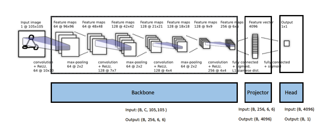
Before we dive further into the structure of this vector space, it will be useful to think of deep learning models as consisting of a backbone, a projector, and a head.

The backbone is the portion of the network that extracts the features (such faces in an image, groups of subject mentions in text, particular words in a sound clip) — often into a high dimensional vector. The role of the projector then is to “filter” that high dimensional vector to suppress features unimportant to the reducing the loss and find combinations of features that are useful. Finally, the “head” of the network uses the refined feature vector to make predictions — usually these predictions are a vector representing the probability of different classes or outcomes.

Often, models trained on huge datasets are fine-tuned by freezing the weights in the backbone and training the projector and head (sometimes these are combined and just called the head of the network as a whole). The idea here is that all the important features for a wide array of tasks is already encoded through the backbone, and we simply need to find good combinations of those features to help perform our task. This falls under the umbrella of “Transfer Learning”.

Today, we will be mapping out these embeddings to understand what kind of vector space they live in, and how different data is separated within it.

Setting up the Data

The wonderful Torchvision package provides us a wide array of pre-trained deep learning models and datasets to play with. These pre-trained models are documented well, with well defined pre-processing steps and architectural hyper-parameters. The datasets are easy to use and help us bypass formatting and writing custom dataloaders. We’re going to start out experiments with the simple MNIST dataset, accessible via the MNIST dataloader in torchvision:

This dataloader will generate two elements for each batch, a batched tensor of images (BATCH_SIZE, 3, 221, 221) and a batched tensor of labels (BATCH_SIZE, 1). We need to resize the images to 221x221 because this is the minimum size accepted by the torchvision pre-trained models. As this is quite large by deep learning standards, we’ll resize them back to smaller dimensions before we visualize them in Tensorboard.

Initializing a Pre-trained Model

Loading a specified pre-trained model architecture in Torchvision is extremely simple:

import torchvision.models as models
vgg16 = models.vgg16(pretrained=True)
vgg16.eval() # Setup for inferencing

We can now generate features for a set of MNIST images with a simple script:

This is perfect for understanding the process of utilizing a pre-trained model to generate embeddings, but to parse these embeddings for use with Tensorboard’s embedding viewer we’ll need a few extra components. We’re going to create a class that does the following:

1. Initializes with a Pytorch model (nn.module object) which can take in a batch of data and output 1 dimensional embeddings of some size
2. Writes paired input data points and their embeddings into provided folders, in a format that can be written to Tensorboard logs

Creating the Tensorboard Writer

The class will need to have methods for generating the embeddings with a model, writing them into files (along with the corresponding data element that produced them), generating a Tensorboard writer object, and using the writer to add embeddings to Tensorboard. We draft the class as follows:

For simplicity the class will not initialize a specific model or dataset for you, since ideally it should work with any model and any dataset as long as the outputs of the model on the dataset are one dimensional embeddings. Note however that certain methods in this class (like create_tensorboard_log()) will need to be modified if data elements are not images or two dimensional arrays. Since we are visualizing embeddings for images, we can take advantage of the “label_img” parameter within the add_embedding() method in TensorboardX to have each embedding be represented by the corresponding image that generated it.

Lastly, we will store both embeddings and data elements as .npy (Numpy array) files with (randomly generated) unique ID’s for each data element. This will allow us to know which data element generated which embedding and easily fetch them as pairs to write into Tensorboard.

Here’s the class:

Generating Embeddings

Now that we’ve learned how to initialize a pre-trained model, a dataset for that model, and written a class to pass all of our outputs to Tensorboard, we can actually start exploring the embedding spaces of different models. Here’s a notebook to do just that:

One thing we need to be cognizant about is that deleting the prediction head of a network is not always straightforward and differs between different model architectures. For example we can delete the prediction head of the VGG-16 model by doing:

vgg16 = models.vgg16(pretrained=True)
vgg16.classifier = vgg16.classifier[0:4] # Remove the pred head

However, for Resnet-152:

resnet152 = models.resnet152(pretrained=True)
class Identity(torch.nn.Module):
    def __init__(self):
        super(Identity, self).__init__()
        
    def forward(self, x):
        return x
resnet152.fc = Identity() # Remove the prediction head

In general, different models have their layers described by different keys and so calling print(model) can sometimes help us understand the structure. Ideally, we only want to get rid of the layer that maps the features to the dimension of a specific dataset (such as the fully connected layer of size 1000 at the end of most torchvision models, which have been pre-trained on ImageNet’s 1000 categories).

After successfully running the notebook above, we can start looking at the structure in some of the embeddings.

From 1000+ Dimensions to 3

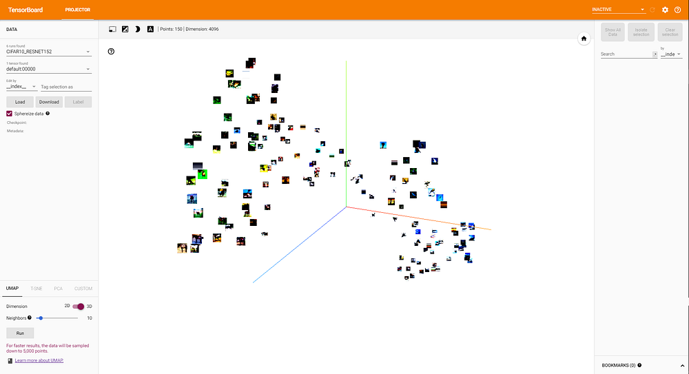
The question that naturally arises is how we can visualize the embeddings generated by our deep learning models when they’re in hundreds or even over a thousand dimensions. The Embedding Projector currently allows for 3 different dimensionality reduction methods to help visualize these embeddings. Here they are with a short and extremely general summary of their overall method (click the links for more information):

Principal Component Analysis: Standardize the data to have 0 mean, calculate eigenvectors for the covariance matrix, order these by largest eigenvalue to get the principal components. The first 3 of these eigenvectors make up the visualization.

T-SNE: Non-linear dimensionality reduction by generating a low dimensional probability distribution where the sampling distances match those in the original space

UMAP: Use cross-entropy and gradient descent to create a low dimensional manifold that shares topological properties with the higher dimensional manifold induced by the data

The default option is PCA, which will often fail to create meaningful clusters in high dimensional embeddings. We can observe for example that in this test (CIFAR10 embedded with Resnet-152), PCA only explains ~26% of the variance in the embeddings (bottom left):

Using the T-SNE algorithm with some tweaking to the perplexity and gradually reducing the learning rate leads to stable clusters

Finally the UMAP algorithm returns much fewer clusters that are distributed wider:

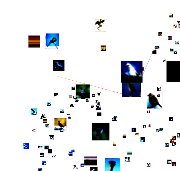
Since the T-SNE result looks the best, we can poke around the space and find interesting images that got mapped to similar portions of the space, for example this small cluster that contains different bird images including ones in flying poses and even just a headshot of an ostritch

or this cluster containing pictures of boats:

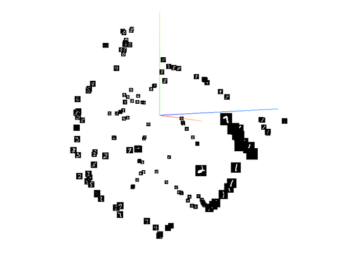
This clustering of classes occurs with MNIST also, here’s Resnet-152 with T-SNE clustering:

Overall, you will find better separation with more powerful models (such as Resnet-152 vs. VGG-16) and datasets that are closer to the original training dataset (Imagenet).

With some experimentation using different model architectures, datasets, and training protocols (such as contrastive learning, which I’ll be writing about soon), you can generate some truly enlightening views of the latent spaces of different deep learning models. Not only does this give you an idea of the functioning of the backbone vs. the head of a network, it also gives you a good look at how networks generalize and parse inputs from different datasets.

Thanks for reading!